Seurat - Guided Clustering Tutorial of 2,700 PBMCs
![]()
This notebook was created using the codes and documentations from the following Seurat tutorial: Seurat - Guided Clustering Tutorial. This notebook provides a basic overview of Seurat including the the following:
- QC and pre-processing
- Dimension reduction
- Clustering
- Differential expression
Downloading data from 10X Genomics
[1]:
system("cd /tmp;\
        wget -q http://cf.10xgenomics.com/samples/cell-exp/1.1.0/pbmc3k/pbmc3k_filtered_gene_bc_matrices.tar.gz;\
        tar -xzf pbmc3k_filtered_gene_bc_matrices.tar.gz")
Setup the Seurat Object
[2]:
library(dplyr)
library(Seurat)
library(patchwork)

# Load the PBMC dataset
pbmc.data <- Read10X(data.dir = "/tmp/filtered_gene_bc_matrices/hg19/")
# Initialize the Seurat object with the raw (non-normalized data).
pbmc <- CreateSeuratObject(counts = pbmc.data, project = "pbmc3k", min.cells = 3, min.features = 200)
pbmc
An object of class Seurat
13714 features across 2700 samples within 1 assay
Active assay: RNA (13714 features, 0 variable features)
[3]:
# Lets examine a few genes in the first thirty cells
pbmc.data[c("CD3D", "TCL1A", "MS4A1"), 1:30]
3 x 30 sparse Matrix of class "dgCMatrix"

CD3D  4 . 10 . . 1 2 3 1 . . 2 7 1 . . 1 3 . 2  3 . . . . . 3 4 1 5
TCL1A . .  . . . . . . 1 . . . . . . . . . . .  . 1 . . . . . . . .
MS4A1 . 6  . . . . . . 1 1 1 . . . . . . . . . 36 1 2 . . 2 . . . .
[4]:
dense.size <- object.size(as.matrix(pbmc.data))
dense.size
709591472 bytes
[5]:
sparse.size <- object.size(pbmc.data)
sparse.size
29905192 bytes
[6]:
dense.size/sparse.size
23.7 bytes
QC and selecting cells for further analysis
[7]:
# The [[ operator can add columns to object metadata. This is a great place to stash QC stats
pbmc[["percent.mt"]] <- PercentageFeatureSet(pbmc, pattern = "^MT-")
[8]:
# Show QC metrics for the first 5 cells
head(pbmc@meta.data, 5)
| orig.ident | nCount_RNA | nFeature_RNA | percent.mt | |
|---|---|---|---|---|
| <fct> | <dbl> | <int> | <dbl> | |
| AAACATACAACCAC-1 | pbmc3k | 2419 | 779 | 3.0177759 |
| AAACATTGAGCTAC-1 | pbmc3k | 4903 | 1352 | 3.7935958 |
| AAACATTGATCAGC-1 | pbmc3k | 3147 | 1129 | 0.8897363 |
| AAACCGTGCTTCCG-1 | pbmc3k | 2639 | 960 | 1.7430845 |
| AAACCGTGTATGCG-1 | pbmc3k | 980 | 521 | 1.2244898 |
[9]:
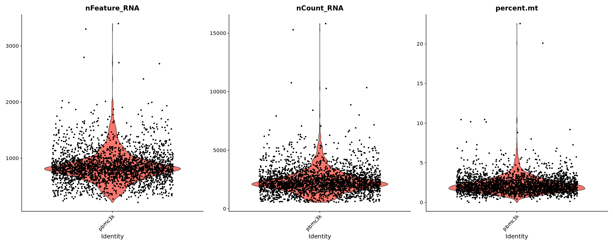
# Visualize QC metrics as a violin plot
options(repr.plot.width=20, repr.plot.height=8)
VlnPlot(pbmc, features = c("nFeature_RNA", "nCount_RNA", "percent.mt"), ncol = 3)
[10]:
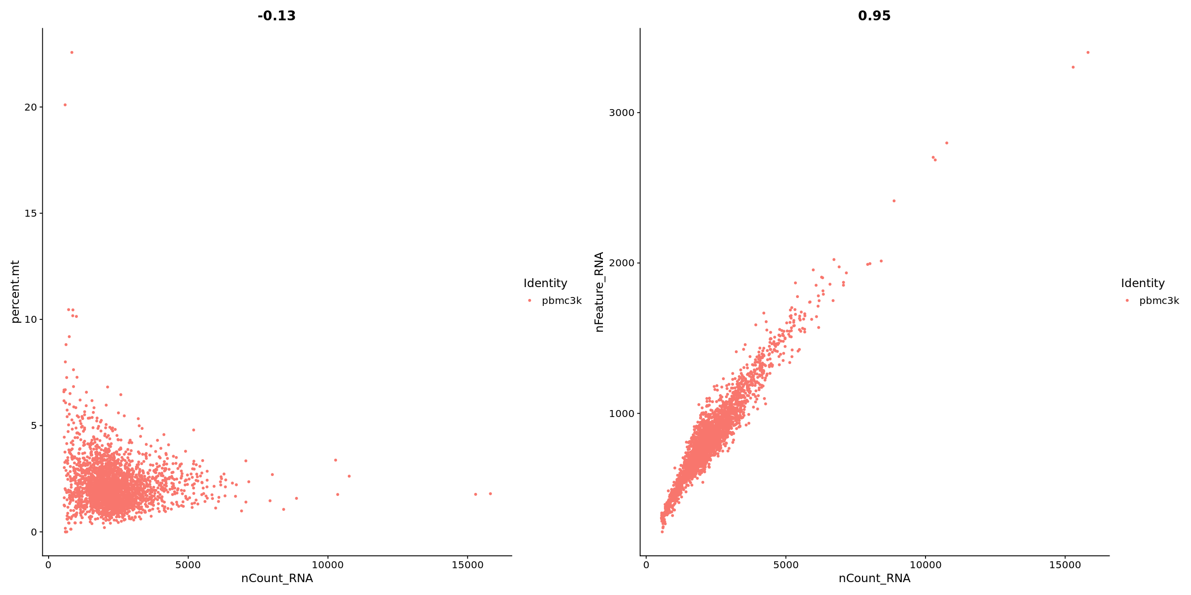
# FeatureScatter is typically used to visualize feature-feature relationships, but can be used
# for anything calculated by the object, i.e. columns in object metadata, PC scores etc.
options(repr.plot.width=20, repr.plot.height=10)
plot1 <- FeatureScatter(pbmc, feature1 = "nCount_RNA", feature2 = "percent.mt")
plot2 <- FeatureScatter(pbmc, feature1 = "nCount_RNA", feature2 = "nFeature_RNA")
plot1 + plot2
[11]:
pbmc <- subset(pbmc, subset = nFeature_RNA > 200 & nFeature_RNA < 2500 & percent.mt < 5)
Normalizing the data
[12]:
pbmc <- NormalizeData(pbmc, normalization.method = "LogNormalize", scale.factor = 10000)
[13]:
pbmc <- NormalizeData(pbmc)
Identification of highly variable features (feature selection)
[14]:
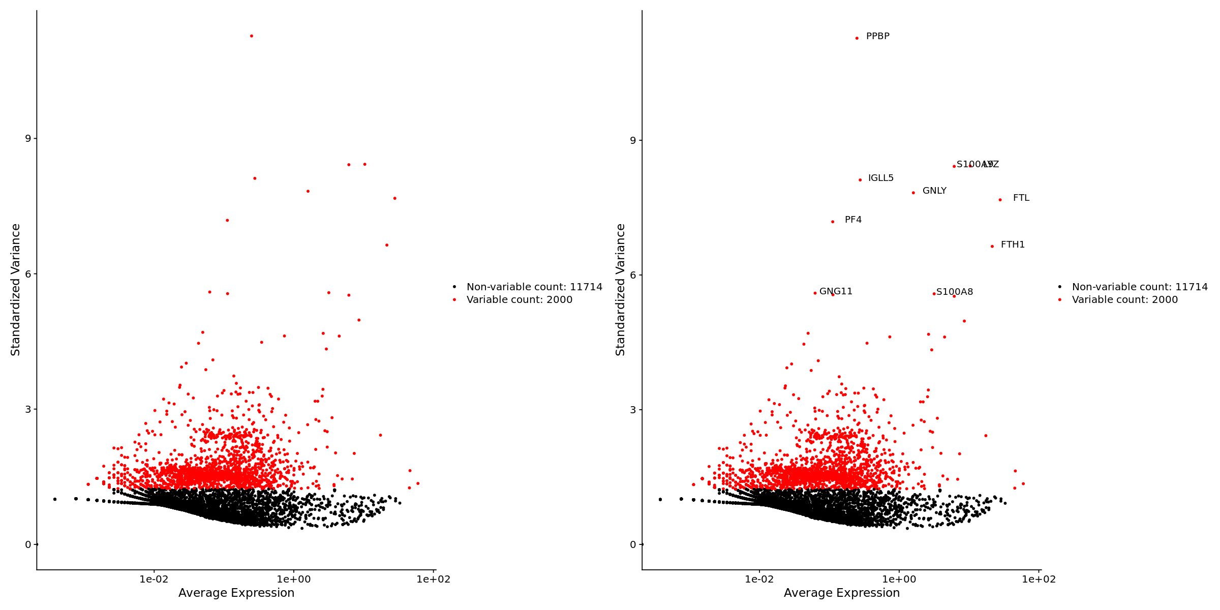
pbmc <- FindVariableFeatures(pbmc, selection.method = "vst", nfeatures = 2000)

# Identify the 10 most highly variable genes
top10 <- head(VariableFeatures(pbmc), 10)

# plot variable features with and without labels
plot1 <- VariableFeaturePlot(pbmc)
plot2 <- LabelPoints(plot = plot1, points = top10, repel = FALSE)
plot1 + plot2
Scaling the data
[15]:
all.genes <- rownames(pbmc)
pbmc <- ScaleData(pbmc, features = all.genes)
Perform linear dimensional reduction
[16]:
pbmc <- RunPCA(pbmc, features = VariableFeatures(object = pbmc))
[17]:
# Examine and visualize PCA results a few different ways
print(pbmc[["pca"]], dims = 1:5, nfeatures = 5)
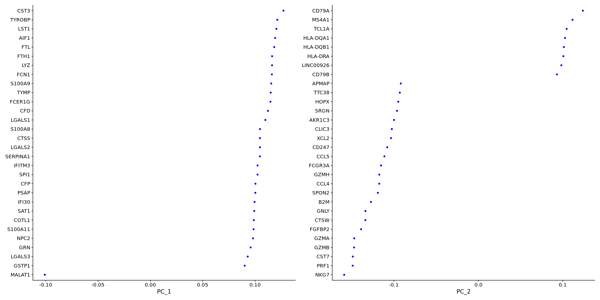
PC_ 1
Positive:  CST3, TYROBP, LST1, AIF1, FTL
Negative:  MALAT1, LTB, IL32, IL7R, CD2
PC_ 2
Positive:  CD79A, MS4A1, TCL1A, HLA-DQA1, HLA-DQB1
Negative:  NKG7, PRF1, CST7, GZMB, GZMA
PC_ 3
Positive:  HLA-DQA1, CD79A, CD79B, HLA-DQB1, HLA-DPB1
Negative:  PPBP, PF4, SDPR, SPARC, GNG11
PC_ 4
Positive:  HLA-DQA1, CD79B, CD79A, MS4A1, HLA-DQB1
Negative:  VIM, IL7R, S100A6, IL32, S100A8
PC_ 5
Positive:  GZMB, NKG7, S100A8, FGFBP2, GNLY
Negative:  LTB, IL7R, CKB, VIM, MS4A7
[18]:
VizDimLoadings(pbmc, dims = 1:2, reduction = "pca")
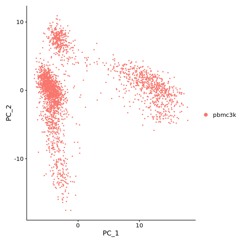
[19]:
options(repr.plot.width=7, repr.plot.height=7)
DimPlot(pbmc, reduction = "pca")
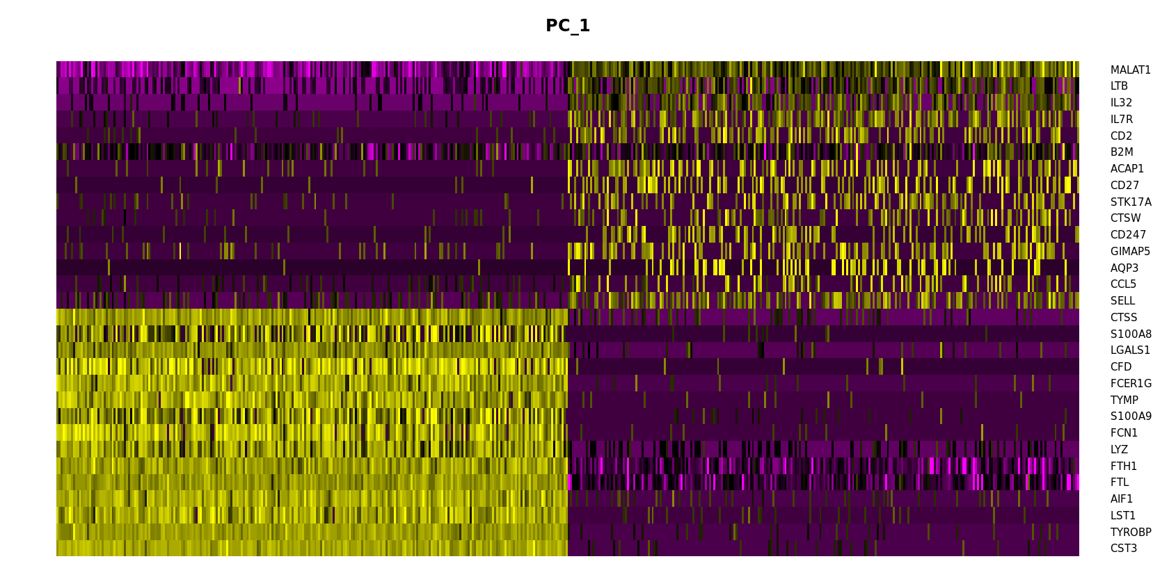
[20]:
options(repr.plot.width=14, repr.plot.height=7)
DimHeatmap(pbmc, dims = 1, cells = 500, balanced = TRUE)
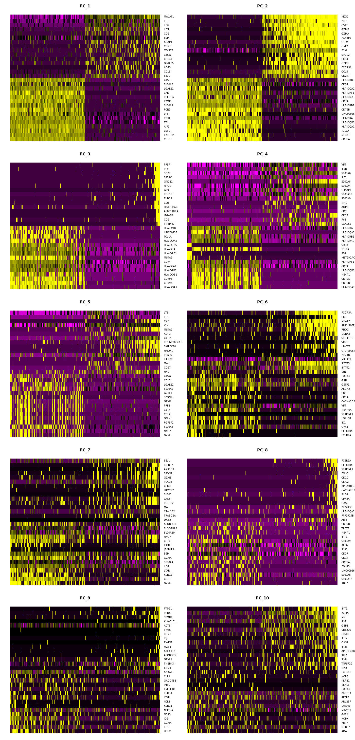
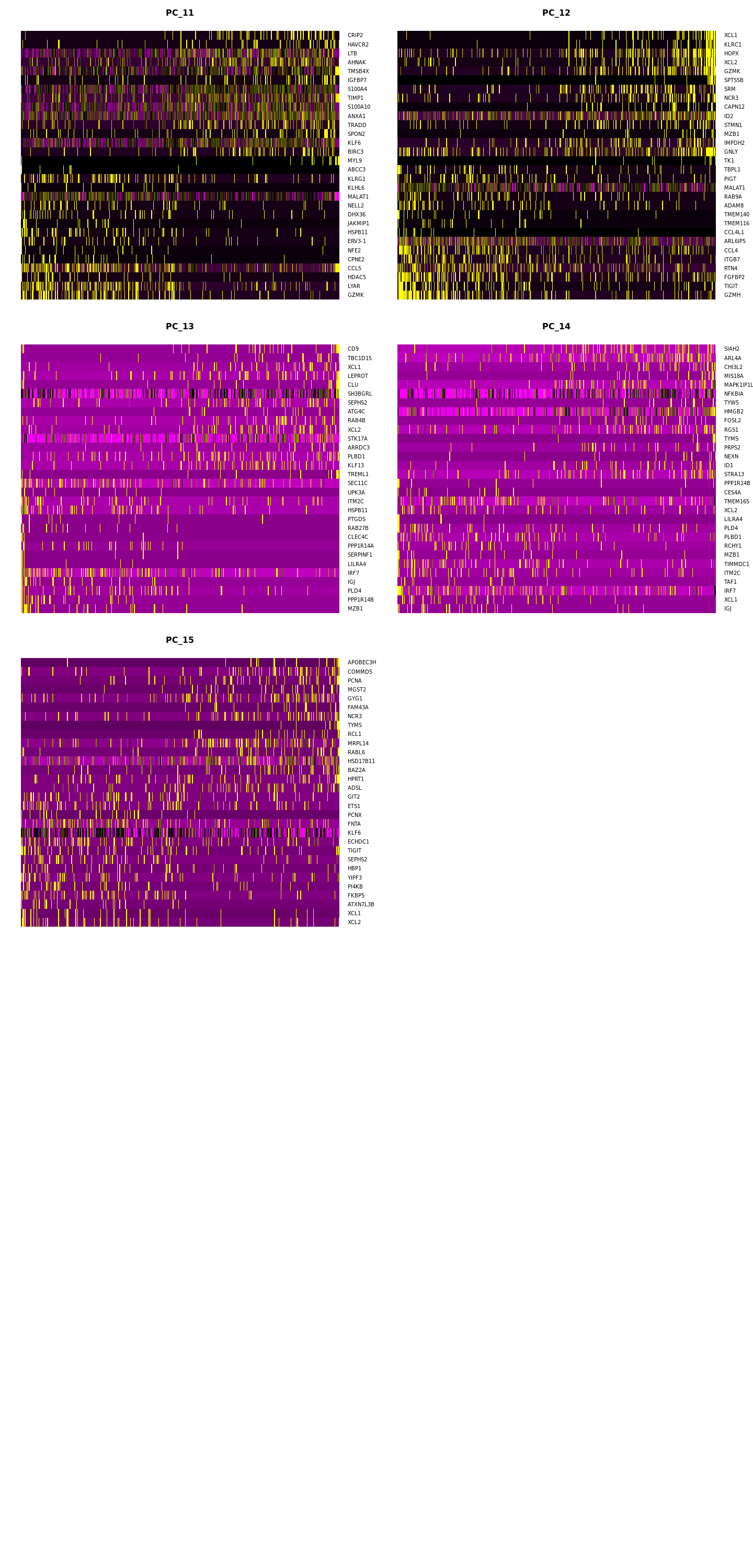
[21]:
options(repr.plot.width=12, repr.plot.height=25)
DimHeatmap(pbmc, dims = 1:15, cells = 500, balanced = TRUE,ncol = 2)
Determine the ‘dimensionality’ of the dataset
[22]:
# NOTE: This process can take a long time for big datasets, comment out for expediency. More
# approximate techniques such as those implemented in ElbowPlot() can be used to reduce
# computation time
pbmc <- JackStraw(pbmc, num.replicate = 100)
pbmc <- ScoreJackStraw(pbmc, dims = 1:20)
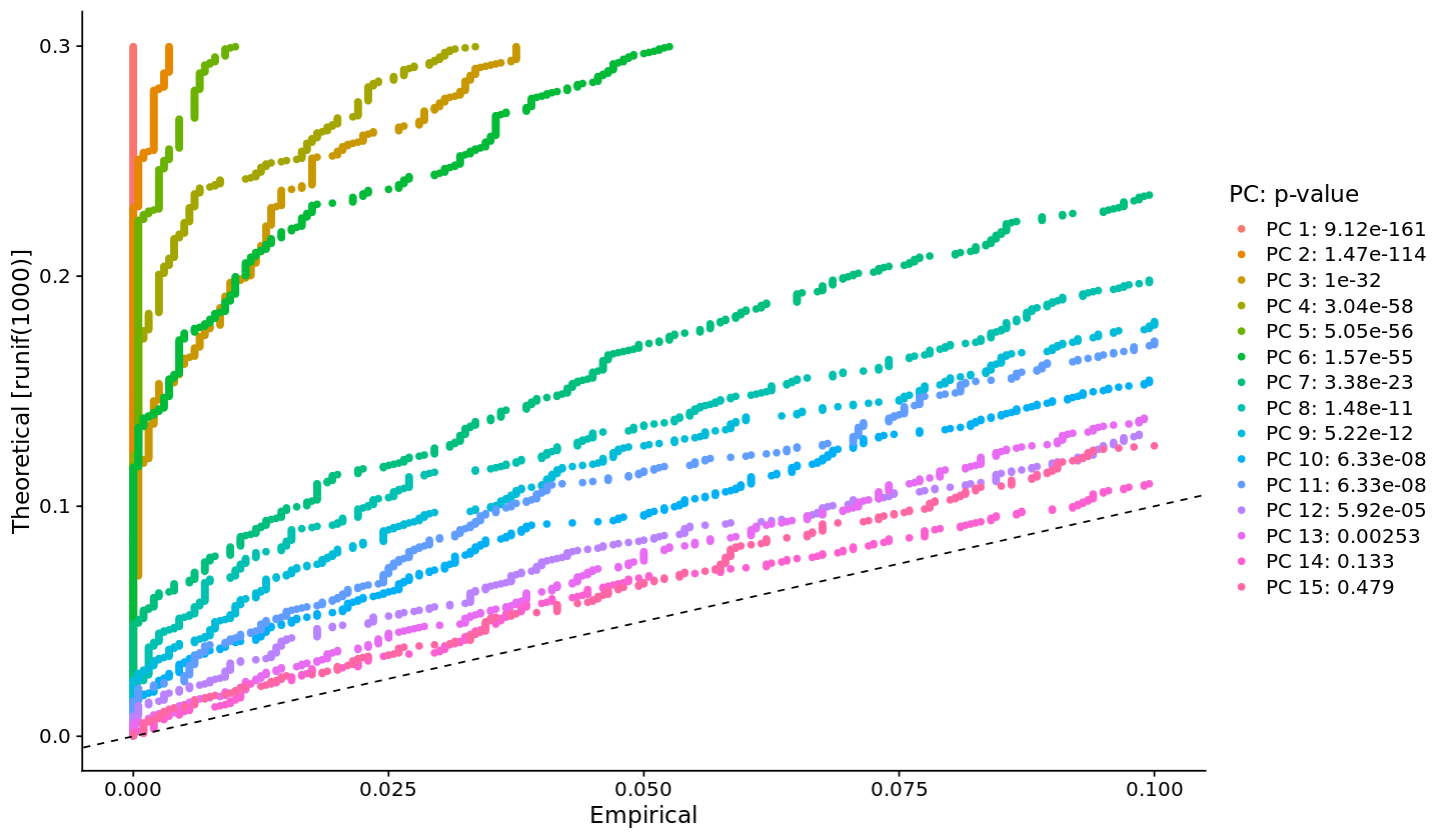
[23]:
options(repr.plot.width=12, repr.plot.height=7)
JackStrawPlot(pbmc, dims = 1:15)
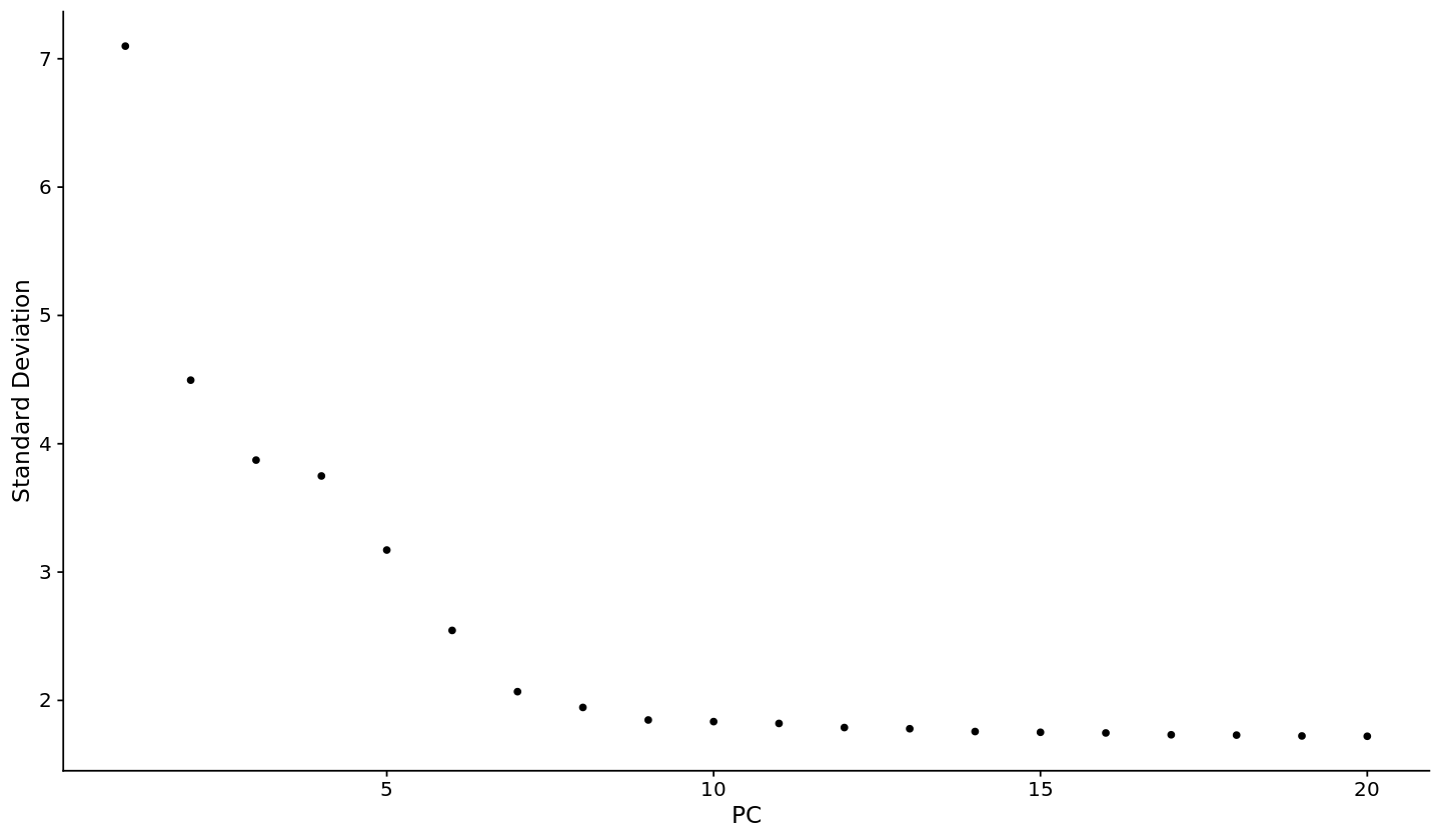
[24]:
options(repr.plot.width=12, repr.plot.height=7)
ElbowPlot(pbmc)
Cluster the cells
[25]:
pbmc <- FindNeighbors(pbmc, dims = 1:10)
pbmc <- FindClusters(pbmc, resolution = 0.5)
Modularity Optimizer version 1.3.0 by Ludo Waltman and Nees Jan van Eck

Number of nodes: 2638
Number of edges: 96033

Running Louvain algorithm...
Maximum modularity in 10 random starts: 0.8720
Number of communities: 9
Elapsed time: 0 seconds
[26]:
# Look at cluster IDs of the first 5 cells
head(Idents(pbmc), 5)
- AAACATACAACCAC-1
- 1
- AAACATTGAGCTAC-1
- 3
- AAACATTGATCAGC-1
- 1
- AAACCGTGCTTCCG-1
- 2
- AAACCGTGTATGCG-1
- 6
Levels:
- '0'
- '1'
- '2'
- '3'
- '4'
- '5'
- '6'
- '7'
- '8'
Run non-linear dimensional reduction (UMAP/tSNE)
[27]:
# If you haven't installed UMAP, you can do so via reticulate::py_install(packages =
# 'umap-learn')
pbmc <- RunUMAP(pbmc, dims = 1:10)
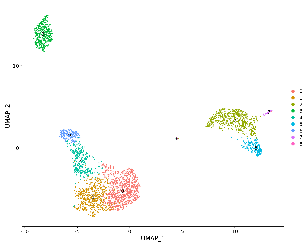
[28]:
# note that you can set `label = TRUE` or use the LabelClusters function to help label
# individual clusters
options(repr.plot.width=10, repr.plot.height=8)
DimPlot(pbmc, reduction = "umap",label=TRUE)
Finding differentially expressed features (cluster biomarkers)
[29]:
# find all markers of cluster 1
cluster1.markers <- FindMarkers(pbmc, ident.1 = 1, min.pct = 0.25)
head(cluster1.markers, n = 5)
| p_val | avg_logFC | pct.1 | pct.2 | p_val_adj | |
|---|---|---|---|---|---|
| <dbl> | <dbl> | <dbl> | <dbl> | <dbl> | |
| IL32 | 1.894810e-92 | 0.8373872 | 0.948 | 0.464 | 2.598542e-88 |
| LTB | 7.953303e-89 | 0.8921170 | 0.981 | 0.642 | 1.090716e-84 |
| CD3D | 1.655937e-70 | 0.6436286 | 0.919 | 0.431 | 2.270951e-66 |
| IL7R | 3.688893e-68 | 0.8147082 | 0.747 | 0.325 | 5.058947e-64 |
| LDHB | 2.292819e-67 | 0.6253110 | 0.950 | 0.613 | 3.144372e-63 |
[30]:
# find all markers distinguishing cluster 5 from clusters 0 and 3
cluster5.markers <- FindMarkers(pbmc, ident.1 = 5, ident.2 = c(0, 3), min.pct = 0.25)
head(cluster5.markers, n = 5)
| p_val | avg_logFC | pct.1 | pct.2 | p_val_adj | |
|---|---|---|---|---|---|
| <dbl> | <dbl> | <dbl> | <dbl> | <dbl> | |
| FCGR3A | 7.583625e-209 | 2.963144 | 0.975 | 0.037 | 1.040018e-204 |
| IFITM3 | 2.500844e-199 | 2.698187 | 0.975 | 0.046 | 3.429657e-195 |
| CFD | 1.763722e-195 | 2.362381 | 0.938 | 0.037 | 2.418768e-191 |
| CD68 | 4.612171e-192 | 2.087366 | 0.926 | 0.036 | 6.325132e-188 |
| RP11-290F20.3 | 1.846215e-188 | 1.886288 | 0.840 | 0.016 | 2.531900e-184 |
[31]:
# find markers for every cluster compared to all remaining cells, report only the positive ones
pbmc.markers <- FindAllMarkers(pbmc, only.pos = TRUE, min.pct = 0.25, logfc.threshold = 0.25);
pbmc.markers %>% group_by(cluster) %>% top_n(n = 2, wt = avg_logFC);
| p_val | avg_logFC | pct.1 | pct.2 | p_val_adj | cluster | gene |
|---|---|---|---|---|---|---|
| <dbl> | <dbl> | <dbl> | <dbl> | <dbl> | <fct> | <chr> |
| 1.963031e-107 | 0.7300635 | 0.901 | 0.594 | 2.692101e-103 | 0 | LDHB |
| 1.606796e-82 | 0.9219135 | 0.436 | 0.110 | 2.203560e-78 | 0 | CCR7 |
| 7.953303e-89 | 0.8921170 | 0.981 | 0.642 | 1.090716e-84 | 1 | LTB |
| 1.851623e-60 | 0.8586034 | 0.422 | 0.110 | 2.539316e-56 | 1 | AQP3 |
| 0.000000e+00 | 3.8608733 | 0.996 | 0.215 | 0.000000e+00 | 2 | S100A9 |
| 0.000000e+00 | 3.7966403 | 0.975 | 0.121 | 0.000000e+00 | 2 | S100A8 |
| 0.000000e+00 | 2.9875833 | 0.936 | 0.041 | 0.000000e+00 | 3 | CD79A |
| 9.481783e-271 | 2.4894932 | 0.622 | 0.022 | 1.300332e-266 | 3 | TCL1A |
| 2.958181e-189 | 2.1220555 | 0.985 | 0.240 | 4.056849e-185 | 4 | CCL5 |
| 2.568683e-158 | 2.0461687 | 0.587 | 0.059 | 3.522691e-154 | 4 | GZMK |
| 3.511192e-184 | 2.2954931 | 0.975 | 0.134 | 4.815249e-180 | 5 | FCGR3A |
| 2.025672e-125 | 2.1388125 | 1.000 | 0.315 | 2.778007e-121 | 5 | LST1 |
| 7.949981e-269 | 3.3462278 | 0.961 | 0.068 | 1.090260e-264 | 6 | GZMB |
| 3.132281e-191 | 3.6898996 | 0.961 | 0.131 | 4.295609e-187 | 6 | GNLY |
| 1.480764e-220 | 2.6832771 | 0.812 | 0.011 | 2.030720e-216 | 7 | FCER1A |
| 1.665286e-21 | 1.9924275 | 1.000 | 0.513 | 2.283773e-17 | 7 | HLA-DPB1 |
| 7.731180e-200 | 5.0207262 | 1.000 | 0.010 | 1.060254e-195 | 8 | PF4 |
| 3.684548e-110 | 5.9443347 | 1.000 | 0.024 | 5.052989e-106 | 8 | PPBP |
[32]:
cluster1.markers <- FindMarkers(pbmc, ident.1 = 0, logfc.threshold = 0.25, test.use = "roc", only.pos = TRUE)
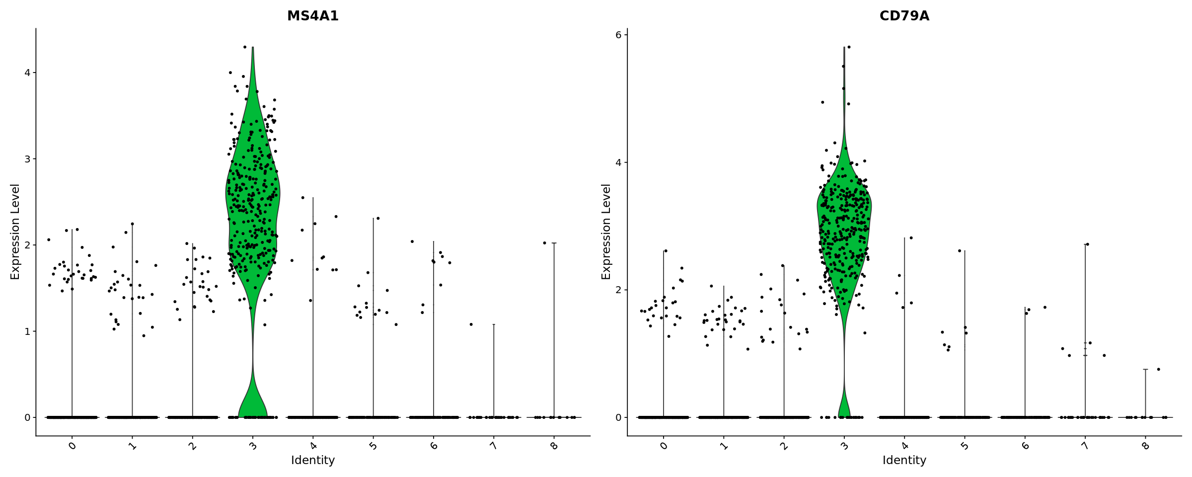
[33]:
options(repr.plot.width=20, repr.plot.height=8)
VlnPlot(pbmc, features = c("MS4A1", "CD79A"))
[34]:
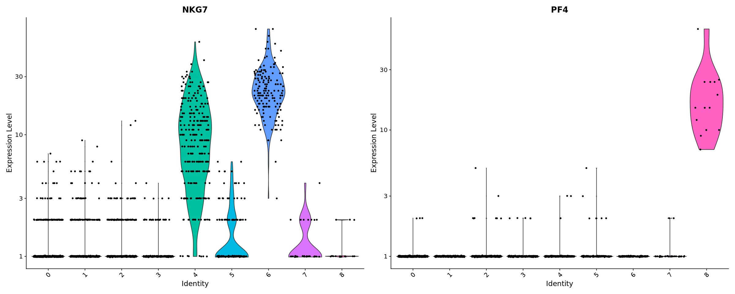
# you can plot raw counts as well
VlnPlot(pbmc, features = c("NKG7", "PF4"), slot = "counts", log = TRUE)
[35]:
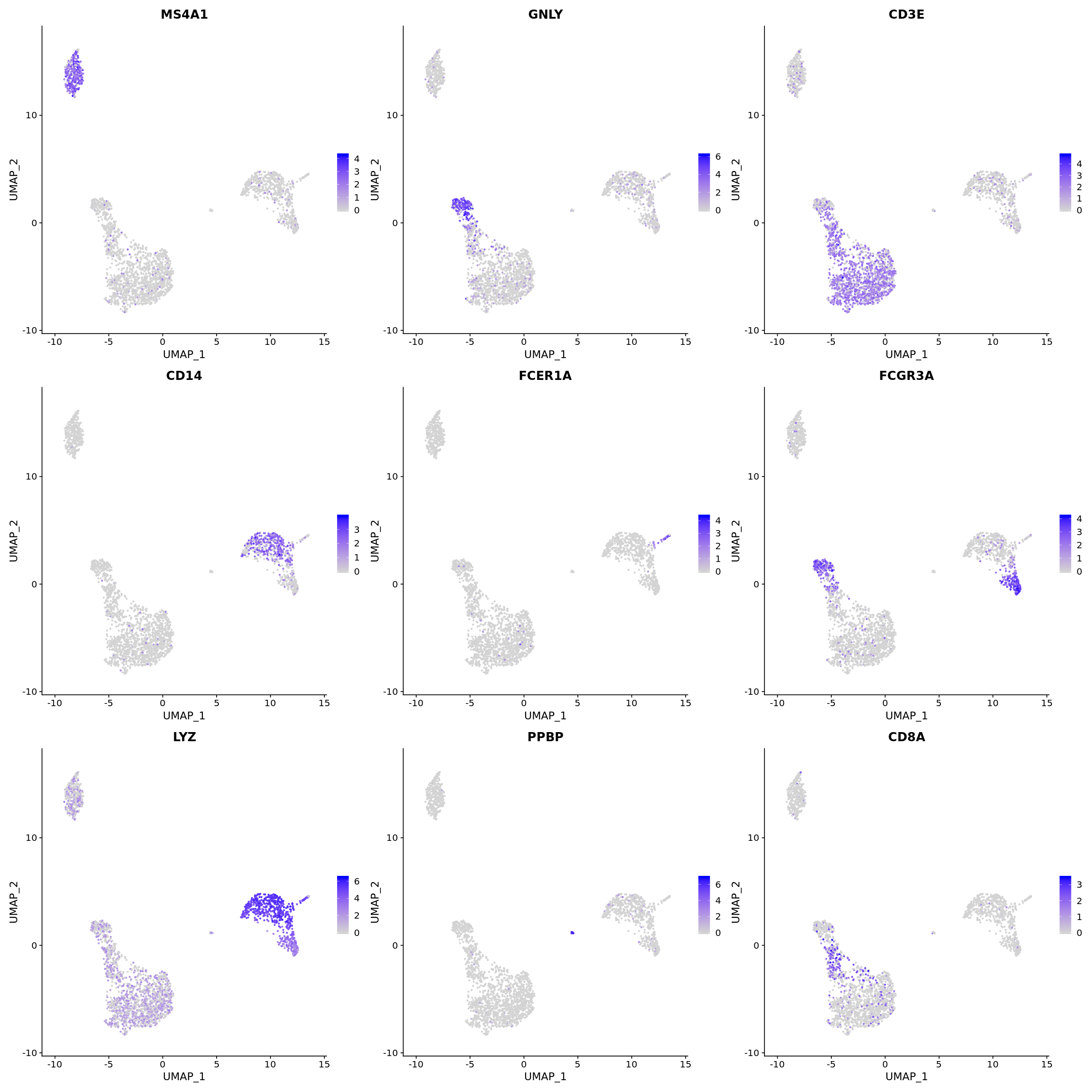
options(repr.plot.width=20, repr.plot.height=20)
FeaturePlot(pbmc, features = c("MS4A1", "GNLY", "CD3E", "CD14", "FCER1A", "FCGR3A", "LYZ", "PPBP",
    "CD8A"))
[36]:
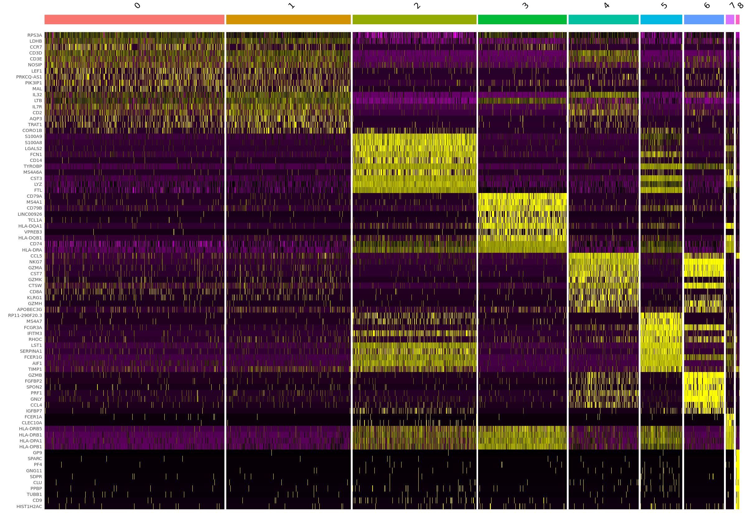
options(repr.plot.width=20, repr.plot.height=14)
top10 <- pbmc.markers %>% group_by(cluster) %>% top_n(n = 10, wt = avg_logFC)
DoHeatmap(pbmc, features = top10$gene) + NoLegend()
Assigning cell type identity to clusters
[37]:
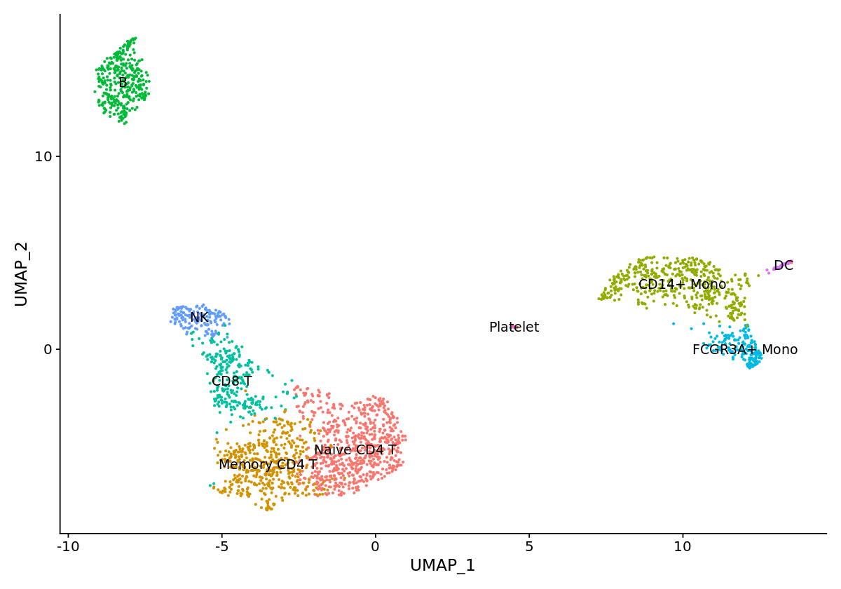
options(repr.plot.width=10, repr.plot.height=7)
new.cluster.ids <- c("Naive CD4 T", "Memory CD4 T", "CD14+ Mono", "B", "CD8 T", "FCGR3A+ Mono",
    "NK", "DC", "Platelet")
names(new.cluster.ids) <- levels(pbmc)
pbmc <- RenameIdents(pbmc, new.cluster.ids)
DimPlot(pbmc, reduction = "umap", label = TRUE, pt.size = 0.5) + NoLegend()
[ ]: